2x2 Mixed Factorial Design
Background information you need to know to understand the 2x2 mixed analysis is covered in the PsychWorld commentary "Within-Subjects Designs" and "2x2 Between Subjects Designs". The mixed factorial design is, in fact, a combination of these two. It is a factorial design that includes both between and within subjects variables. One special type of mixed design, that is particularly common and powerful, is the pre-post-control design. This is a design in which all subjects are given a pre-test and a post-test, and these two together serve as a within-subjects factor (test). Participants are also divided into two groups. One group is the focus of the experiment (i.e., experimental group) and one group is a base line (i.e., control) group. So, for example, if we are interested in examining the effects of a new type of cognitive therapy on depression, we would give a depression pre-test to a group of persons diagnosed as clinically depressed and randomly assign them into two groups (traditional and cognitive therapy). After the patients were treated according to their assigned condition for some period of time, let’s say a month, they would be given a measure of depression again (post-test). This design would consist of one within subject variable (test), with two levels (pre and post), and one between subjects variable (therapy), with two levels (traditional and cognitive) (Figure 1).
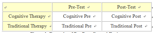
Figure 1. Example of Pre-Post-Control Design
When a researchers uses the pre-post-control design he or she is usually looking for an interaction such that one cell in particular stands out, and that is the experimental group’s post test score. Ideally the pre-test scores will be equivalent. It is the post-test score difference between the experimental and control group that is important (see Figure 2).
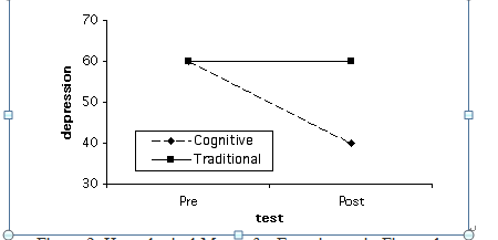
Figure 2. Hypothetical Means for Experiment in Figure 1
Therefore, in terms of post-hoc tests the most important comparison is between the post-test mean for the experimental group and the post-test mean for the control group (see Figure 3).
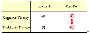
Figure 3. Comparison of Post-Test Means
Also, it is typical for the experimenter to expect a change in the experimental group from pre to post, but not in the control group, which would make the important post-hoc comparisons between pre- and post-test for the experimental groups and between pre- and post-test for the control group (see Figure 4).
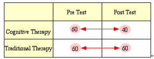
Figure 4. Comparison of Pre vs. Post Test Means for Both Groups
Of course, the pre-post-control design is not the only type of mixed design. Another common type of mixed design (and within-subjects design in general) is one that includes a change over time, so that one independent variable consists of multiple measures of one group of people over time. So, for example, we might be interested in comparing the interest of males vs. females in math and science over some time period during development. More specifically, we could give a group of school children a measure of interest in math and science at age 10 and then give the same group of students the same measure of interest at age 18. Our design then would look like Figure 5, and one set of possible means would look like the means in Figure 6, which would represent an interaction.
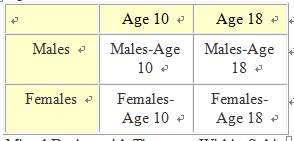
Figure 5. Mixed Design with Time as a Within-Subjects Factor
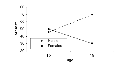
Figure 6. Hypothetical Means for the Experiment in Figure 5
The two-way mixed analysis of variance is the most complex type of design/analysis that is covered in the PsychConnections.com modules. The VirtualStatistician and experimental psych modules cover the inferential tests listed below. Although, of course, there are many more types of statistical tests, there are an amazing number of experiments, both within psychological and biological sciences that you can answer with the designs/analyses listed below. Of course, there are many variations, since the examples in the modules are limited to two levels of the independent variables and two independent variables, but adding levels and independent variables is just a slight extension of what is covered. There are also cases in which there are no continuous variables, in which case you would often use a "non-parametric" technique, and complex modeling of many continuous variables which would require "multivariate" analyses. However, in cases where an experimenter uses a traditional method, in which groups are formed and variables are manipulated the designs and analyses covered in these modules will often work fine. Further, these more complex types of data analyses such as multivariate techniques are extensions of the basic "univariate" techniques coverd in the modules, so that this knowledge can serve as an important and necessary foundation for the understanding of these techniques.
(Figure 7 is a map/flow chart to aid you in selecting the appropriate analysis for a given design among those covered in the PsychConnections.com modules. If you want to go to the module to review a given analysis click on the appropriate white square.)

Figure 7. Flow Chart Representing Choice of Analysis Depending on Design
|
2x2 Between Subjects Factorial Design
Design This module covers the types of designs and analyses involving more than one independent variable. This gets tricky because it’s difficult when you first begin this exercise to differentiate between adding an additional level to an existing independent variable, as compared to adding a new independent variable all together. For example, let’s say that we are interested in studying the effect of room temperature on test taking. To do this we compare test scores of students who take a test in a 90 degree room vs. those who take a test in a 50 degree room. This is a case of one independent variable (i.e., room temperature) and two levels (i.e., 50 and 90 degrees), and the appropriate analysis would be a between-subjects’ t-test (assuming the two groups are made up of two separate groups of students). Let’s extend this design by adding a third group, 70 degrees. We now have an experiment with one independent variable (i.e., room temperature) and three levels (50, 70, and 90 degrees). We have not added an additional independent variable; rather we have simply added a third level to the already existing independent variable. It is crucial that you understand the difference between a variable and a level in order to select and interpret the analysis for a given experiment. So how would we go about adding a second independent variable? Remember that a variable, by definition, must have at least two levels (i.e., it must "vary"). To keep our discussion of the complex concept of multi-factor designs at the most basic level, we will consider the simplest type of situation where there are more than one independent variables; the 2 X 2 ("two by two") between-subjects factorial design. In our example with room temperature, let’s go back to the original two groups (50 vs. 70 degrees), but let’s add a new independent variable with two levels, test difficulty (difficult vs. easy). Note that this new variable is qualitatively different than room temperature, and it has levels of it’s own, so that we've done more than simply add an additional level to the existing independent variable. Since this is a between-subjects design we will randomly assign subjects to four groups, as illustrated in Figure 1. Experiments that include multiple categorical independent variables and a continuous variable are often called "factorial" designs, and the independent variables are called "factors" (not to be confused with a "factor analysis", which is a multivariate statistical technique, which involves the statistical grouping of multiple continuous variables.) 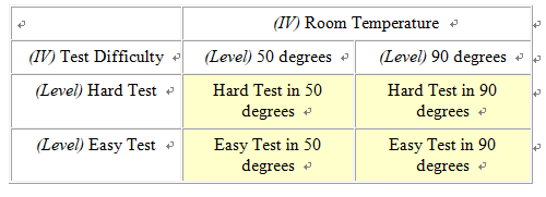 Figure 1. Example of a 2 X 2 Design Whenever we see numbers and the multiplication sign in describing designs like this (2 X 2 or "two by two"), each of the numbers represents an independent variable and the value of the number represents the number of levels of that independent variable. For example, 3 x 2 would mean two independent variables, one with three levels and one with 2. 3 X 4 X 2 would represent an experiment with three independent variables, one with three levels, one with 4, and one with 2. Researchers often use the term "way" to refer to the number of independent variables in an analysis, so a "one-way" ANOVA refers to an ANOVA with one independent variable, and a two-way ANOVA would be used to analyze an experiment with two independent variables. Mathematically, we can analyze data with as many independent variables as we want. However, due to the complexity of interpreting higher level ANOVAs, it’s rare to see anything beyond a three-way ANOVA. Results and Analyses An experiment that includes multiple categorical independent variables and one continuous dependent variable is appropriately analyzed using an analysis of variance (ANOVA). Statistically, in a two-way ANOVA there are three basic types of effects that are tested: main effect for independent variable A, main effect for independent variable B, and effect for the interaction of A and B. We will consider main effects first. A main effect for a given independent variable means that there is a significant difference between the levels of this independent variable across levels of the other independent variable. Another way of thinking of this is that there is an effect for one independent variable regardless of the the level of the other. For example, in the test experiment, students are probably going to do better on the easy test than the hard, regardless of the temperature of the room they are tested in (Figure 2 displays means that represent such an effect, and Figure 3 is a line graph of these means). The mean of the means for a given independent variable, collapsing across the levels of another independent variable, are referred to as "marginal means" and these means aid us in interpreting a main effect. So, if we look at the marginal means in this example we can see that there is clearly a dramatic difference between the marginal means associated with test difficulty (60 vs. 80) and no difference in the means associated with room temperature. 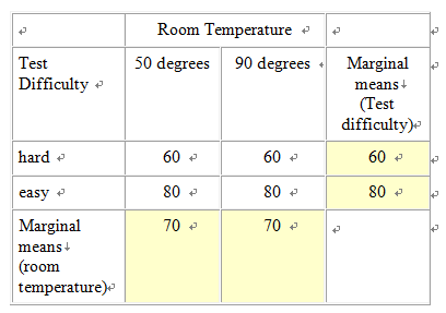 Figure 2. Means representing a main effect for Test Difficulty. 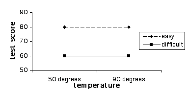 Figure 3. Line graph of means from Figure 2 We could, of course, find a main effect of Room Temperature, by reversing this hypothetical example, in which case we could, for example, change the means for both test difficulty groups in the 50 degree room to a score of 60, and for both test difficulty groups in the 90 degree room to a score of 80. The examples thus far might lead you to the conclusion that a main effect for one independent variable precludes the possibility of finding a main effect for the other. Actually this is not true as illustrated in the table and line-graph in figures 4 and 5. Notice that in this case, we would conclude from the results that students perform best in 90 degrees regardless of whether the test was hard or easy, and they also perform better on the easy test regardless of whether they take it in 50 degrees or 90. Note that the graphs of the means in both figures 3 and 5 represent parallel lines. Parallel lines in these types of graphs indicate that there are main effects in the results, but no interactions. If the lines are not parallel this is indicative of an interaction. (Note that it is possible to find both a significant main effect and a significant interaction with the same set of means, and in this case, the lines will not be parallel. In interpreting such a case, the main effect is usually ignored, in that it is misleading. We will address this further below.) 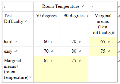 Figure 4. Means Representing a Main Effect for Both Room Temperature and Test Difficulty. 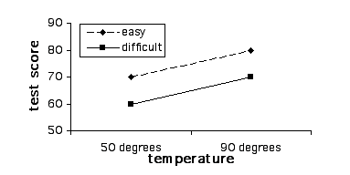 Figure 5. Line Graph of Means from Figure 4 Figure 6 and 7 represent the classic "crossing" interaction. This effect is an interaction because the effect of one independent variable depends on, the effect of the other. If we found these means, and we were asked a question about one independent variable, such as: "Did students do better with the hard test or easy test?", our answer would be something like: "That depends, with room temperature of 50 they did better on the hard test, with room temperatures of 90 they did better on the easy test". Conversely, if someone asked: "Did students do better in ninety degrees or 50 degrees?", your answer would be: "That depends, with the hard test they did better in 50 degrees, with the easy test they did better in 90 degrees." As you can see from the marginal means there is absolutely no main effects in this case. This illustrates the fundamental advantage of using a multi-way design and analysis. If we were to set up and experiment where we just compared hard vs. easy tests or 50 vs. 90 degree rooms, and students scored just as is illustrated below, we would never realize that the effect of one of these factors was dependent on the other. Likewise if we analyzed the present experiment, and students scored just as illustrated below, just using two t-tests, one for each of the independent variables, our conclusions would be quite different about the effect of these two independent variables, and our conclusions would be incorrect. 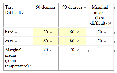 Figure 6. Means Representing "crossing" Room Temperature X Test Difficulty Interaction 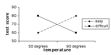 Figure 7. Line Graph of Means from Figure 6 Although the classic "crossing" interaction in figures 6 and 7 is used most often to illustrate an interaction in a two-way analysis, it’s also possible to find an interaction in which the lines do not cross (though note they are still not-parallel), such as illustrated in figures 8 and 9. Note that, to explain the results, we would still have to describe the results of one independent variable in terms of the other. For example: "Do students do better on hard tests or easy tests?" "It depends, in a fifty degree room there is no difference, but in a ninety degree room they do much better on easy tests." Note that this also represents the case that I referred to above in which the marginal means indicate that there are two main effects. When we average across effects for room temperature, the mean for the ninety-degree room is higher, and when we average across effects for test difficulty, the easy test scores are higher. However, clearly if we were to conclude from these results that students do better in ninety degree rooms, regardless of test difficulty, or that they do better on easy tests regardless of room temperature, we would clearly be incorrect. The correct conclusion to be drawn from the results below is that students do best when the test is easy and the temperature is 90 degrees. Otherwise temperature and difficulty level doesn't matter. This is why researchers often disregard a main effect that occurs in the data analysis when there is also an interaction. 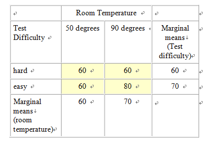 Figure 8. Means Representing a non-crossing Room Temperature X Test Difficulty Interaction 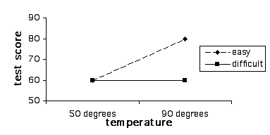 Figure 9. Line Graph of Means from Figure 8 |

8장, 9장
제 8 장
실험 참가자들을 나누는 2가지 방법을 크게 Between-subjects design과 Within-subjects design으로 나눌 수 있다. Between-subjects design은 독립변수의 수준에 노출되는 실험 참가자들이 각각 다르지만 within-subjects design의 실험 참가자들은 동일하다. Between-subjects design의 장점은 실험참가자들이 각각 다른 수준에 노출되므로 수준들 끼리의 행동에 영향을 받지 않는다. 이 외에도 실험 참가자들이 노출되는 수준이 하나 이므로 시간이 적게 걸린다거나 한 실험 session에서 많은 자료를 얻을 수 있다. 단점으로는 수준에 따라 나누어지는 집단이 일정하지 않아서 행동이 한쪽으로 치우칠 수 있는 가능성이 있다. 그러나 이런 가능성은 random assignments가 해소 시킬 수 있다. Within-subjects design은 실험 참가자들의 수가 적게 필요한데 반면 심각한 단점으로는 한 실험참가자가 하나의 독립변수 수준에 노출 되면 노출 이전의 상태로 돌리는 것이 불가능하다. 이와 같은 순서에 따른 오염이 있을 수 있는데 이와 같은 효과를 최소화 하는데 counterbalancing과 같은 방법이 있다.
Counterbalancing을 사용하고자 하면 각기 다른 독립변수의 수준에 똑같이 confounding effect를 배분하여야 한다. 많이 사용되는 ABBA counterbalancing은 두 개의 수준이 어떤 시행에 해당되어 배분되는지를 나타낸다. 실험 참여자들은 모든 시행을 다 해내되 그 수준의 시행 순서를 조절하여 counterbalancing을 맞춘다. 하지만 이런 것이 가능하게 하는 Counterbalancing의 가정이 존재하는데 그것이 바로 confounding effects가 선형을 이룬다는 것이다. Confounding effect가 선형을 이룬다는 조건하에 ABBA counterbalancing은 within-subjects design의 confounding effect를 제거하는 것이 가능하다.
또 다른 counterbalancing에는 symmetrical transfer를 가정하는 counterbalancing이 존재하는데 symmetrical trasfer라 함은 독립변수의 수준의 순서가 A뒤에 B가 오는 순서와 B뒤에 A가 오는 순서의 역이라는 가정에서 출발하는 것이다. 이 가정에 위배되는 asymmetrical transfer가 발생하면 이 counterbalacing은 소용이 없다.
독립변수의 수준이 많아 질수록 complete counterbalancing 설계들은 더 복잡해지며 partial counterbalancing을 이용하여 몇 개의 순서들을 임의로 선택하는 방법을 이용하기도 한다. Partial counterbalancing 중에서 독립변수의 수준이 두 수준 이상일 때 Latin square를 이용한다. 각 수준이 시행되는 순서에서 똑같은 빈도로 나타나고 각 수준에서 먼저 제시되거나 뒤에 제시되는 수준 역시 같은 빈도로 나타난다.
그러나 이러한 Counterbalancing에 의해서도 교정 되어질 수 없는 within-subjects design의 또 다른 단점은 range effects이다. 학습 곡선에서 그 효과가 역 U형태를 띄는 것처럼 중간에서 최고 수준의 수행능력을 가지는데 range effect가 이처럼 within-subjects experiment의 결과로 나올수 있다.
Matched-group design을 이용하면 within-subjects experiment의 장점을 이용할 수도 있고 개인적 차이의 문제도 어느 정도 피할 수 있다. 이 방법은 독립변수의 각 수준의 참가자들을 유사하게 할당하는 것이다. Matching을 통하여 독립변수가 행동의 변화를 야기했다고 할 때 그것이 틀릴 수 있는 가능성을 감소 시킬 수 있다. 이 말은, 종속변수에서의 차이가 독립변수에 의해서 발생하였다는 가능성을 더 많이 지지하는 것이다.
제 9 장
이 챕터에서는 single-variable experiments와 multiple-variable experiments, factorial experiments를 살펴본다.
Single variable experiments에서 독립변수가 두개의 수준을 가지는 실험은 가장 단순한 실험의 하나로 볼 수 있다. 두 개의 수준에 experimental group과 control group이 노출된다. 두 개의 수준을 가지는 실험은 독립변수 자체의 가치에 대해서 알아낼 수 있는 수단이 되며 결과를 해석하고 분석하기 쉽다. 또한 어떤 이론이 타당한지를 살펴보는 적절한 방법이기도 하다. 그러나 독립변수와 종속변수 사이의 관계의 형태를 알려주지는 못하는 단점이 있다. 대부분 심리학 함수에서 ceiling effects와 floor effect라고 부르는 것이 있는데 ceiling effects는 종속변수가 어떤 수준을 넘어설 수 없을 때 발생한다. Floor effects는 실험참가자가 더 이상 그 이하로는 반응할 수 없는 값을 일컫는다. 또한 어느 수준이 ceiling인지 floor인지 명확히 할 수 없는데 이런 것 들을 피하기 위해서 두 개의 수준 실험에서 실험 수준들이 interpolate 혹은 extrapolate 하지 않도록 해야 한다. 또한 두 개의 수준 실험은 경쟁 이론들을 제거하는데 도움이 되지 못한다. 이의 결과로는 여러 경쟁 이론들 중 어느 것이 더 적합한지 판단이 어렵기 때문이다.
Multilevel experiment의 경우는 독립변수의 수준이 셋 이상인 경이며 독립변수와 종속변수의 함수적 관계를 설명한다. 장점은 결과가 실험의 관계적 본성을 추론하는데 도움을 준다는 것이다. 두 개의 수준 실험보다는 훨씬 더 많은 정보를 제공하고 있다고 사려된다. 여러 수준의 실험을 하면 변수들간의 관계를 살펴보기 용이하며 수준이 많아 질수록 독립변수와 종속변수 사이의 함수적 추론이 가능하다. 또한 더 많은 수준일수록 독립변수의 범위는 현실적이며 그 결과를 보여줄 수 있을 만큼 충분해야 한다는 조건을 만족시키기 쉽다. 단점은 시간과 노력이 많이 든다는 것이다. 실험을 분석하는 통계적 검증도 더 어려워지고 해석도 까다롭다.
실제 실험에서는 하나 이상의 독립변수가 포함된 실험이 많다. 이런 실험에 빈번하게 이용되는 factorial design 설계를 살펴보자. Factorial design은 각 요인들의 수준의 조합으로 이루어진다. Factorial design에서 요인들은 실험 참가자들 내에서 혹은 실험 참가자들 간의 변인이 될 수 있고 이러한 두 종류의 요인이 하나의 실험에 모두 포함되면 mixed factorial design이라고 한다. Factorial design의 장점은 interaction을 살펴보는데 용이하다. interaction이라 함은 하나의 독립변수와 참가자의 행동 사이에서의 관계가 두 번째 독립변수의 수준을 결정 지을 때 발생한다. 두 번째 장점은 더 많은 상황들이 요인으로 만들어졌고 그것들이 어떤 수준에서 어떻게 효과가 발생하였는지를 보여주기 때문에 실험이 복잡해지는 대선 가능한 많은 상황에 대해 일반화 하는 것이 가능하다. 세 번째 장점은 요인으로 만들 수 있는 상황이 더 많을수록 variability의 추정치는 더 작아진다. Variability의 추정치가 작아질수록 우리가 발견하는 통계적 유의성이 높아진다. Factorial design의 단점으로는 시간과 비용이 많이 들고 결과를 해석하는 것이 어렵다. Factorial design의 분석을 위해서는 Analysis of variance가 요구되는데 이를 위해서 충족되어야 하는 여러가지 가정들을 실험이 끝날때까지도 발견해 내지 못하는 경우가 많다.
많은 논문들이 연속적인 일련의 실험 결과를 보고 한다. 이는 많은 연구자들이 converging series design을 선택하기 때문이다. 이는 점진적 해결의 실험들을 지칭하기도 하며 대부분 single-variable이나 small factorial experiments로 구성된다. 점진적인 실험들의 설계로 중요 변수들을 변화시키는 방법은 실용적인 문제에 대한 해결법을 제시하는 것이 가능하다.
Converging operation 접근은 검토할 수 있는 많은 가설들을 가지고 실험을 시작하고 실험이 수행되는 과정에서 가설을 제거하여 결국 설명력 있는 하나의 가설로 수렴하는 방법이다. 이 기법의 장점은 많은 선택의 여지를 제공하고 중간에 새로운 독립변수나 새로운 수준을 선택하는 등 능률적으로 이루어진다. 또한 실험 설계자체가 반복되므로 결과에 대한 신뢰도가 높다. 그러나 실험내의 변수들간의 상호작용을 파악하기 어렵고 이를 파악하고자 하면 factorial design을 해야 한다. 두 번째로 일련의 실험의 결과를 분석하는데 있어서 하나의 실험과 다른 실험을 비교하는 것이 between subjects design으로 행해지므로 그에 수반되는 단점을 다 가지게 된다. 마지막 단점은 앞선 실험의 결과를 분석하는데 시간이 많이 걸린다는 단점이 있다. 그러나 이러한 converging operation design은 응용 및 기초 연구모두에 효율적이고 능동적인 방법이다.
[Chapter 8]
- 참가자를 할당하는 두 가지 방법
(1) between subject design: 최소 두 명의 참가자들간에 조작되는 방법
(2) within subject design: 한 명의 참가자 내에서 변인이 조작되는 방법을 말한다.
- between subject design의 장점은, 참가자들이 독립변인의 한 수준에만 노출되므로 다른 수준에는 영향을 받지 않는 다는 것이다. 최소 두 명의 인원인 참가자는 단 하나의 수준에만 노출됨으로 다른 수준에는 영향을 받지 않는다. 이에 반해, between subject design의 단점은 피실험자 간에 독립변인의 각 수준에 할당되는 집단이 다른 수준에 할당되는 집단과 동등하지 않을 가능성도 배제할 수 없다는 것이다.
- within subject design의 장점은, 실험에 참가하는 인원이 적어도 실험이 가능하다는 것이다. 또한, 독립변인의 여러 수준으로부터 수집된 자료 표본들에서 발견된 차이가 실제로 발생했는지 추측해 통계적 검증을 해야 한다. within subject design은 변산성이 적기때문에 독립변인의 수준간의 차이가 실제 차이라고 믿게 될 가능성이 높다. 이에 반해, within subject design 단점은, 어떤 효과를 실험하는 동안 체계적으로 변할 수 있다. 따라서 순서효과가 발생할 가능성을 인지하고 독립변인이 순서에 의해 오염되지 않도록 해야 한다.
- within subject design의 단점인, 순서효과를 줄여줄 수 있는 방법으로 counterbalancing시켜야 한다. ABBA counterbalancing는 한 참가자 내에서 순서효과를 통제할 수 있지만, 그 순서효과가 선형적이라는 가정을 할 수 있어야 한다. 그러나 여기서도 조건들 간의 대청적 전이에 대한 가정이 있어야 한다. 비대칭전이가 발생되면, counterbalancing은 효과적이지 못하다. 그 외에도 각 수준들이 각 위치에 동일한 횟수만큼 나타나도록 하면서 몇몇 순서들만을 임의로 선택하는 partial counterbalancing가 있다.
- 또 다른 방법으로, matched-groups design은 독립변인의 각 수준에 유사란 참가자들을 할당시키는 것이다. 이는 독립변인에 의해 행동에서의 차이가 발생되었다고 말하는 것이 틀릴 확률을 감소시킨다. 게다가 matched-groups design은 종속변인에서의 차이가 우연적으로 발생된 것이 아니라 독립변인에 의해 일어날 가능성이 높아지기 때문에 통계적인 이점도 제공해 준다.
[Chapter 9]
- Single variable experiments
(1) Two level experiments: 하나의 독립변인이 두 개의 수준을 가지는 실험으로, 실험집단과 통제집단으로 나누어 두 수준에 노출시킨다. 이 방법은 독립변인이 연구로써의 가치가 있는지 확인할 수 있으며, 결과를 해석하고 분석하기 용이하다는 장점이 있다. 하지만, 이렇게 두 개의 수준 사이의 거리가 명확하지 않고, 천장효과나 바닥효과의 수준이 어디인지 분명하게 나눌 수 없는 단점이 있다.
(2) Multilevel experiments: 독립변인의 수준이 세 개 이상인 실험으로, 이 실험 방법은 하나의 실험에서 세 수준만 포함되어 있어도 각 변인들의 관계에 대해 두 개 수준의 실험보다 많은 정보를 제공해 준다는 장점이 있다. 하지만, Two level experiments에 비해 많은 시간과 노력이 요구된다. Multilevel experiments을 분석하기 위한 통계기법을 통한 검증도 더 어려울뿐아니라 데이터를 해석하는 것도 더 복잡해진다.
- Factor design은 하나의 독립변인의 각각 수준을 두 번째와 세 번째 독립변인의 각 수준과 매치시키는 요인적인 결합이다. Factor design은 정확도의 감소 없이 일반화 가능성을 증가시킬 수 있으며, 특히 상호작용을 연구할 수 있다는 장점이 있다. 이러한 상호작용은 한 독립변인과 참가자의 행동 사이의 관계가 두 번째의 독립변인 수준에 따라 달라질 때 발생된다. 또한, 상황을 또 하나의 독립변인으로 만들어 결과에 대한 정확성과 일반화 가능성을 증가시킬 수 있다. 하지만, Factor design은 시간과 비용측면의 단점을 가지고 있으며, 결과를 해석하는 것 또한 어렵다는 단점이 있다.
- Converging series design은 남아있는 하나의 가설이 주어진 자료를 설명할 수 있을 때까지 가설들을 점진적으로 제외시켜 나갈 수 있는 수렵조작을 발견하도록 해준다. 장점으로는 큰 요인실험보다 융통성이 크고, 반복실험이 내재되어 있어 실험결과가 반복될 수 있는 것임을 증명할 때마다 권위를 높일 수 있다. 특히, Factor design에 비해 유연성이 높은 이점이 있지만, 상호작용을 평가하기 어렵고, 다름 실험을 하기 전에 이전 실험을 분석해야 하는 단점을 가지고 있다.
'공부하기 > 경영학과 군사학' 카테고리의 다른 글
| 상위 산업/업종 코드표 & 산업/업종 코드표 (0) | 2020.12.01 |
|---|---|
| HS코드 (0) | 2020.11.30 |
| 사업계획서의 골격체계(Outline of Business Plan) [사업계획서 작성요령] (0) | 2020.11.26 |
| 사업계획서 작성요령 (0) | 2020.11.26 |
| ◈ 사업계획서 작성 요령 (0) | 2020.11.26 |


댓글